PUFAnalytics, a complete guide to evaluating PUFs in the browser and in Python
A tour of PUFAnalytics, the open-source toolkit for physically unclonable functions. It covers every view of the web app, how each metric is computed, how the browser and Python give bit-identical results, and a full reference of the Python API.
, 25 min read
A paper about a new physically unclonable function (PUF) has to report the same handful of numbers: uniformity, uniqueness, reliability, bit-aliasing, an identification error rate, some randomness tests, and how much error correction a key would need. Almost every group computes them with its own scripts, and the scripts quietly disagree. Some report uniqueness as twice the standard value. Some quote a false-acceptance rate of zero because none of their few hundred comparisons failed. Some run NIST tests on a few hundred bits, where the p-values mean nothing.
PUFAnalytics is my attempt to make that part of the work boring and correct. It is a Python package and a web app that give the same answers to the last digit. You can load measurements or simulate a population, get every standard metric with confidence intervals, and leave with a LaTeX table, figures and a script that reproduces it all. It accompanies our IEEE APCC 2025 paper.
Try it: open the PUFAnalytics web app and press Explore a demo population. Nothing is uploaded; it runs in your browser and works offline. The code is on GitHub under the MIT license.
New to PUFs? How a PUF works explains the hardware, the four headline metrics and how PUFs are attacked. This post is about the tool: what each part does, how to use it, and how the numbers are computed.
Contents
- Two engines, one answer
- The data model
- The evaluation pipeline
- A tour of the web app, one view at a time
- Reproducibility: same seed, same bits
- Using the Python package and the command line
- Full Python API reference
- How it is tested, limits and how to cite
Two engines, one answer
PUFAnalytics exists twice. The Python package (pip install, NumPy only) suits scripts, notebooks, batch jobs and the command line. The web app is plain HTML, CSS and JavaScript modules with no framework and no build step; it suits exploring a data set, making figures and showing results to someone. Its analysis engine in web/js/core/ is a line-by-line port of the Python modules, and it runs in a Web Worker so the page stays responsive during a 1,000-sample bootstrap.
Scroll sideways to see the whole diagram.
Two decisions keep the engines in step:
- One random number generator for both. Simulators and the bootstrap draw from xoshiro128**, seeded through SplitMix32, implemented identically in Python and JavaScript. Neither engine uses
Math.random()or NumPy’s generator. - A parity test in CI.
tests/make_golden.pywrites reference values from Python intoweb/tests/golden.json, andnode web/tests/parity.test.mjsrequires the browser engine to reproduce all of them. That is over 2,400 checks across metrics, statistics, NIST tests and simulators.
Your data stays with you. The web app is a static site on GitHub Pages. Files are parsed and analysed on your machine and saved only in your browser’s IndexedDB, and a service worker caches the app so it keeps working offline.
The data model
Everything in PUFAnalytics works on one structure, PUFDataset: a block of devices × measurements × bits, plus an operating-condition label (such as 25C or 85C) for each read-out. Measurement 0 of each device is its enrolment reference. Every metric is one particular comparison inside this block:
Scroll sideways to see the whole diagram.
reference="majority", the bitwise majority of all reads). Note how the 85 °C reads flip more bits: that is what the per-condition BER measures.| Comparison | Metric | Ideal |
|---|---|---|
| Share of 1s in a device’s reference | Uniformity | 50% |
| One bit position across all devices’ references | Bit-aliasing | 50% at every position |
| Reference vs reference, over all device pairs | Uniqueness (inter-device distance) | 50% |
| A device’s re-reads vs its own reference | Reliability, bit error rate (BER) | 100%, 0 |
| The same, split by condition label | BER per operating condition | as low as possible |
Data formats
The importer accepts CSV, TXT, JSON and NumPy .npy. The richest layout is one row per read-out, with the response in binary or hex:
device,measurement,condition,response
chipA,0,25C,0xA3F1C29B7E4D0516
chipA,1,85C,0xA3F1C2997E4D0716
chipB,0,25C,0x5C0E3D64819BF2E9
Simpler layouts also work:
- one response per line (one device each);
device,response, where repeated device rows are re-measurements;device,measurement,response;- whitespace-separated bits;
- NumPy arrays shaped
(devices, bits)or(devices, measurements, bits).
Separators can be commas, semicolons, tabs or spaces, and # starts a comment. In auto mode a file is read as binary only if every response is made of 0s and 1s; otherwise it is hex, at 4 bits per digit. Method notes: data formats.
The evaluation pipeline
A full evaluation answers six questions in order and then writes them up. The web app’s sidebar follows the same order, so working down it top to bottom covers everything.
Scroll sideways to see the whole diagram.
A tour of the web app
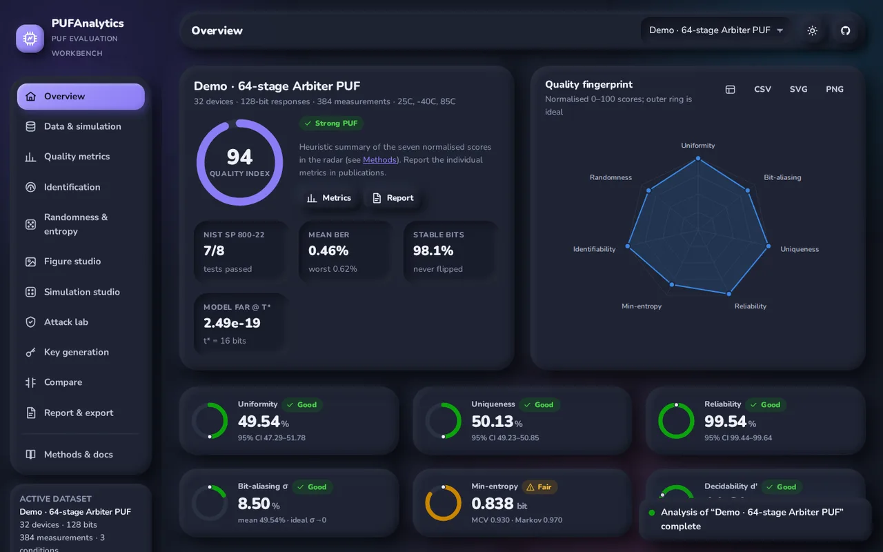
Open the app. With no data loaded, the overview offers two ways in:
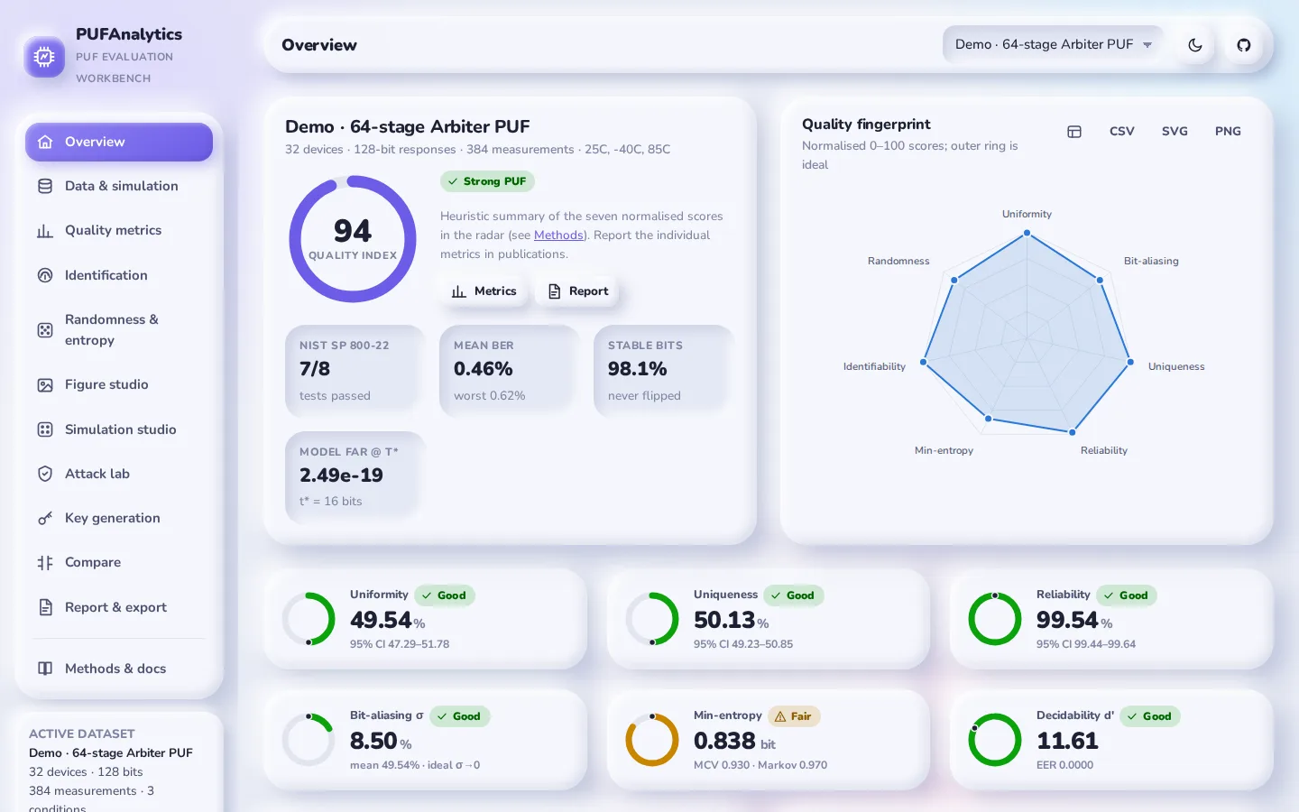
- Explore a demo population simulates 32 Arbiter PUF devices (64 stages, 128 challenges each). Each device is read 4 times at each of three conditions (25 °C, −40 °C and 85 °C), with noise scaled 1×, 1.8× and 2.6×.
- Import your data takes you to the import panel.
The rest of this section goes through the views in sidebar order. All screenshots show the demo population, so you can follow along. Each view has a Method notes link to the part of the app’s built-in documentation that defines what it computes.
Some controls are common to every view:
- The dataset picker in the top bar switches between loaded data sets.
- The moon button toggles dark mode.
- Every chart has CSV, SVG and PNG buttons, and a table icon that shows the numbers behind it.
1. Data & simulation
This is where data comes in, either simulated or imported.
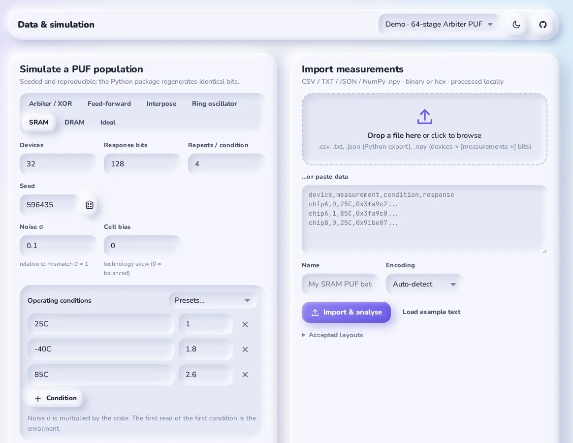
To simulate a population:
- Pick a model tab.
- Set the Devices, Response bits, Repeats / condition and Seed fields. The dice button draws a random seed.
- Set the model’s own parameters, in the row below.
- Add operating conditions with + Condition, or pick one from Presets. Each condition has a label and a noise scale. The first read of the first condition is the enrolment.
- Press Generate & analyse.
Seven models are built in:
| Model | What it simulates | Parameters (defaults) |
|---|---|---|
| Arbiter / XOR | Additive delay model: the response is the sign of a weighted sum of challenge-parity features; XOR of several chains | stages 64, XOR chains 1, noise σ 0.05 |
| Feed-forward | Arbiter PUF where intermediate arbiters set later challenge bits (non-linear) | stages 64, loops 1, noise 0.05 |
| Interpose | (x, y)-iPUF: an x-XOR arbiter’s output is inserted mid-challenge of a y-XOR arbiter | stages 64, x 1, y 1, noise 0.05 |
| Ring oscillator | Pairs of oscillators compared by frequency, with process variation and a systematic gradient shared by all chips | process σ 1, noise 0.1, gradient 0, pairing neighbour/disjoint |
| SRAM | Power-up state of each cell from a fixed mismatch plus thermal noise | noise 0.1, cell bias 0 |
| DRAM | Retention: a cell reads 1 if it decays during the refresh pause; heat speeds decay | noise 0.1, threshold 0, temperature shift 0.3 |
| Ideal | Uniform random bits with independent flips: what “perfect” looks like at your sample size | flip probability 0.02 |
The Ideal model is more useful than it looks. With 32 devices, even a perfect PUF will not show exactly 50% uniqueness, and simulating an ideal population of the same size shows you how much scatter to expect. Method notes: simulators.
To import:
- Drop a file on the drop zone, or paste text into the box.
- Give it a name and choose an encoding: Auto-detect, Binary or Hexadecimal.
- Press Import & analyse.
Load example text fills the box with a valid sample, and Accepted layouts lists every format.
Below the two panels, every loaded data set has Rename, CSV, JSON and delete buttons. Under those are three pre-processing tools and a response explorer:
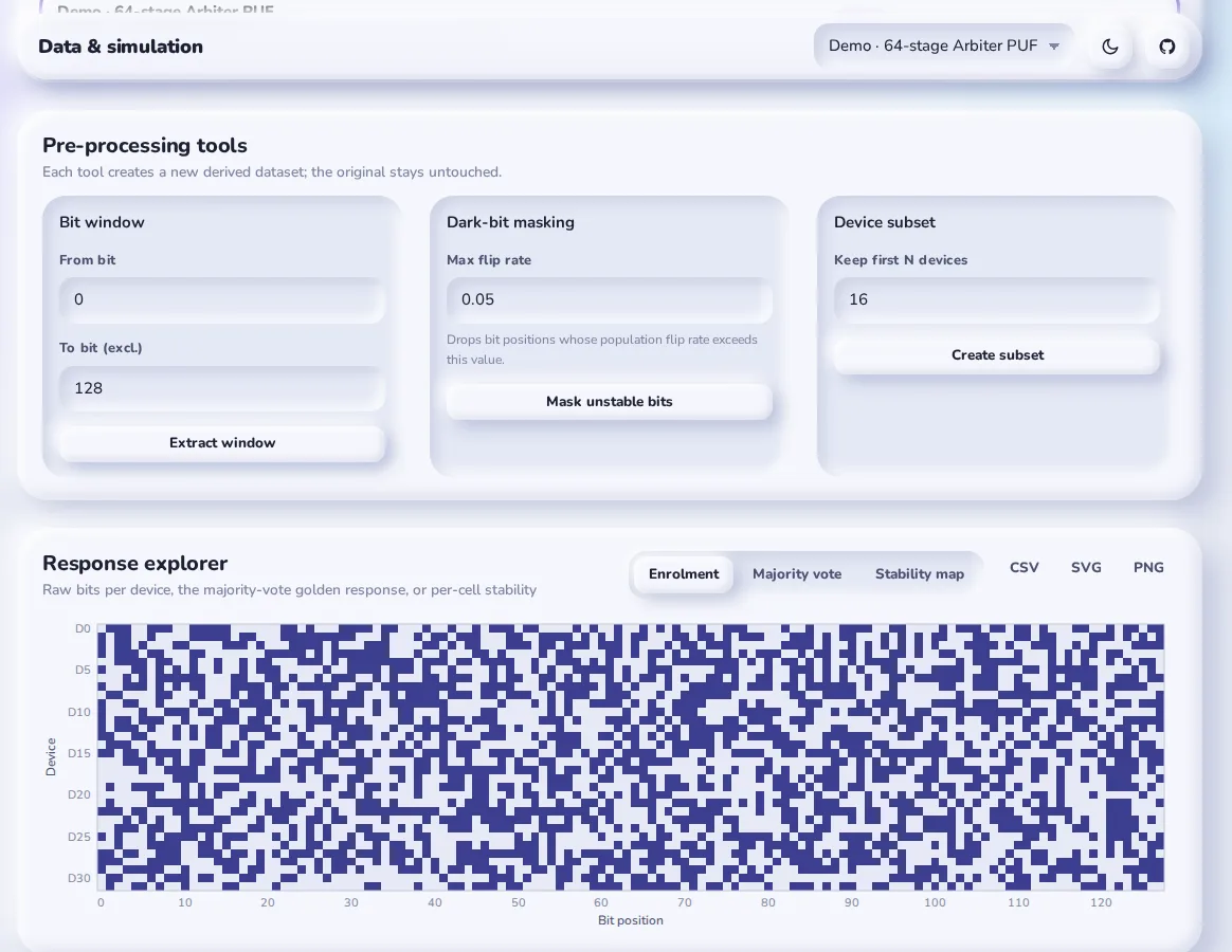
The pre-processing tools never change the original. Each one creates a new, derived data set:
- Bit window keeps the bit positions from From bit up to, but not including, To bit. Use it, for example, to study the first 64 bits of a 128-bit response.
- Dark-bit masking drops bit positions whose flip rate across the population is above a threshold (default 0.05). This is the standard way to trade response length for reliability before key generation.
- Device subset keeps the first N devices. It is useful for checking how stable a metric is as the population grows.
The response explorer draws every device’s bits as a bitmap. It has three modes: Enrolment, Majority vote (the bitwise majority of all reads) and Stability map (the flip rate of each cell). Stripes or columns in the enrolment view mean bias, and bright cells in the stability map show where the noise is.
In Python: pa.simulate(), pa.PUFDataset.from_file(), PUFDataset.subset() and quality.bit_flip_rate().
2. Quality metrics
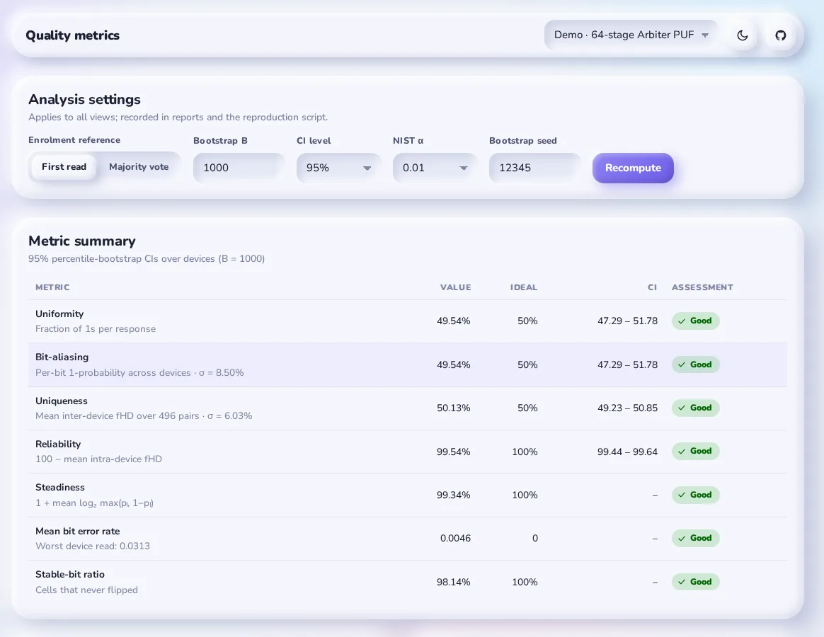
Analysis settings apply to every view, and the report and reproduction script record them:
- Enrolment reference. First read (measurement 0) or Majority vote (the bitwise majority of all reads, a “golden” response).
- Bootstrap B. The number of bootstrap resamples for the confidence intervals. The default is 1,000; 0 turns them off.
- CI level. 90%, 95% or 99%.
- NIST α. The significance level of the randomness tests. The default is 0.01, as NIST recommends.
- Bootstrap seed. Makes the intervals reproducible.
Press Recompute after changing any of them.
The summary table gives each metric with its ideal value, interval and an assessment. Below it are bar charts per device and per bit position, plus the error rate of every bit position. For k devices with n-bit references Ri and T re-reads Ri,t:
Here HW is the Hamming weight (number of 1s) and HD the Hamming distance (number of differing bits). Steadiness measures how consistently each cell of a device reads the same value. With pi,l the share of 1s that bit l of device i gives over its reads:
The confidence intervals resample devices, not bits. The interval should describe what happens if you had built a different batch of chips, and the chip is the unit of variation. For uniqueness, a device paired with its own duplicate in a resample is skipped, so it cannot create artificial zero distances. The demo gives uniqueness 50.13% with a 95% interval of 49.23 to 50.85, and reliability 99.54% (99.44 to 99.64).
One historical note: PUFAnalytics versions before 2.0 returned uniqueness as twice the mean inter-device distance (ideal 1.0 instead of 0.5). Version 2.0 fixed this, and the changelog says so, because a value copied from an old version into a new paper would be wrong by a factor of two.
Method notes: quality metrics. In Python, the pufanalytics.quality module has one function per metric.
3. Identification
Can a reader tell device A from device B, given one noisy read? This view treats the PUF like a biometric.
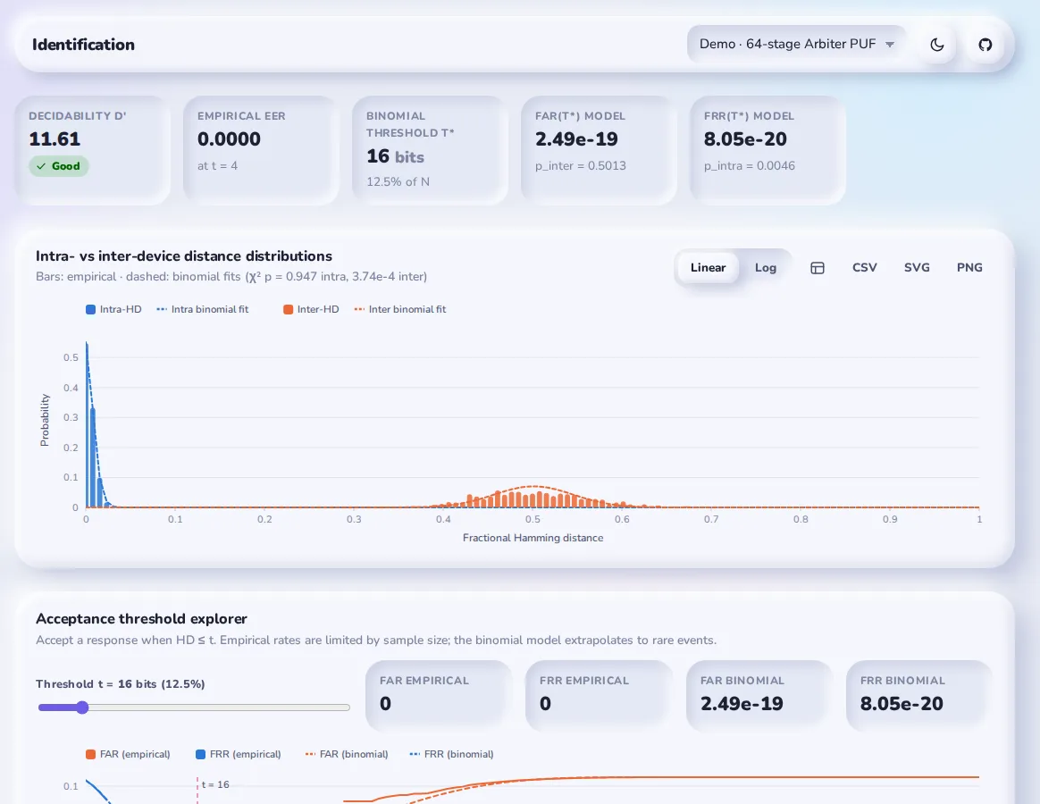
The histogram puts the two distributions side by side. The intra-device distances (a device against its own re-reads) sit near zero. The inter-device distances (device against device) sit near 50%. The further apart they are, the easier identification is. Three numbers summarise the gap:
- Decidability d′ is the distance between the two means, in units of their pooled spread: . Above about 6, errors are practically absent. The demo gives 11.61.
- Empirical EER is the equal error rate read directly off the measured distances.
- Binomial FAR and FRR model the distances as Binomial(n, p), with p fitted to each distribution.
A reader accepts a response when its distance to the enrolled one is at most t bits. Then the false-acceptance rate is FAR(t) = P(inter-distance ≤ t), and the false-rejection rate is FRR(t) = P(intra-distance > t). PUFAnalytics picks the optimal threshold t* that minimises the larger of the two.
The binomial model matters because measured data cannot show small error rates. The demo has 32 devices, so it has only 496 inter-device pairs, and the smallest non-zero FAR it could ever measure is about 1 in 500. The model extrapolates: at t* = 16 bits it gives FAR = 2.49 × 10⁻¹⁹.
Those tails are summed in log space, so they stay accurate below 10−300 rather than rounding to zero. A χ² goodness-of-fit p-value appears next to each fit, so you can see whether the binomial assumption holds for your data. The chart below shows the model’s main lesson for design: the error falls exponentially with response length.
Show the numbers
| Length | 1% BER | 5% BER | 10% BER | 15% BER |
|---|---|---|---|---|
| 16 bits | 2.1e-3 | 1.1e-2 | 3.8e-2 | 7.9e-2 |
| 32 bits | 1.6e-5 | 8.7e-4 | 3.5e-3 | 1.6e-2 |
| 48 bits | 3.1e-7 | 3.1e-5 | 6.6e-4 | 3.4e-3 |
| 64 bits | 1.8e-9 | 2.7e-6 | 1.1e-4 | 8.0e-4 |
| 96 bits | 3.6e-13 | 9.7e-9 | 1.8e-6 | 6.6e-5 |
| 128 bits | 7.8e-17 | 3.6e-11 | 5.4e-8 | 5.8e-6 |
| 192 bits | 6.8e-25 | 5.6e-16 | 3.0e-11 | 2.8e-8 |
| 256 bits | 3.6e-32 | 9.1e-21 | 1.7e-14 | 1.8e-10 |
stats.identification_vs_length(). Empirical rates can never show anything this small: 32 devices give only 496 inter-device pairs, so the smallest error you can observe directly is about 1 in 500.The acceptance threshold explorer has a slider for t. It shows the empirical and model FAR and FRR at the chosen threshold, and draws all four curves on a log axis. Further down are a DET curve (FRR against FAR, the standard biometric plot) and the inter-device distance matrix. A dark cell off the diagonal there means two devices that are suspiciously alike.
Method notes: identification. In Python: stats.decidability(), stats.far_frr_curve(), stats.binomial_far_frr(), stats.binomial_fit() and stats.identification_vs_length().
4. Randomness & entropy
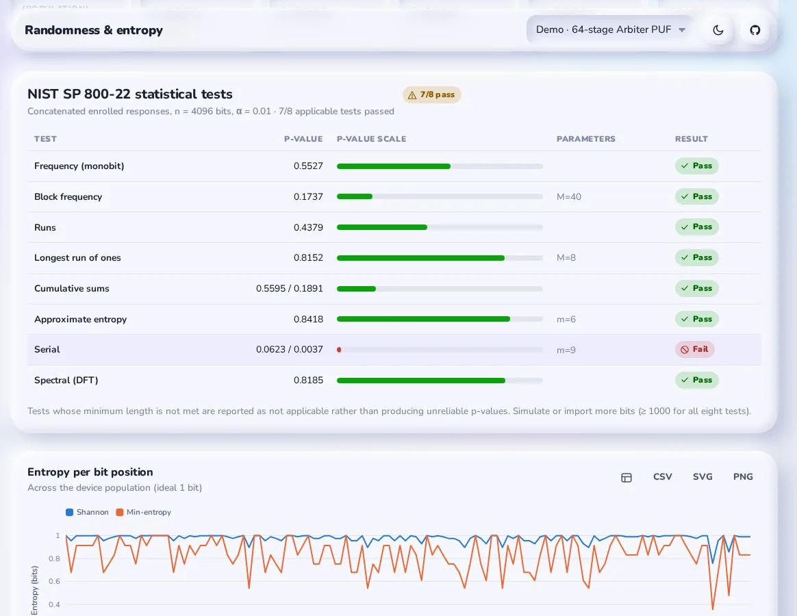
The enrolled responses of all devices are joined into one bit stream and run through eight tests from NIST SP 800-22:
| Test | What it looks for | Minimum length |
|---|---|---|
| Frequency (monobit) | too many 1s or 0s overall | 100 bits |
| Block frequency | imbalance within blocks of M bits | 100 |
| Runs | too many or too few runs of identical bits | 100 |
| Longest run of ones | unusually long runs inside blocks | 128 |
| Cumulative sums | drift of the running ±1 sum (forward and backward) | 100 |
| Approximate entropy | over-frequent m-bit patterns | depends on m |
| Serial | uneven frequencies of all overlapping m-bit patterns (two p-values) | depends on m |
| Spectral (DFT) | periodic structure | 1,000 |
The implementations reproduce the worked examples in the NIST standard to six decimal places. The spectral test uses an exact DFT for any length, through Bluestein’s algorithm, rather than padding to a power of two.
A test that does not have enough data says not applicable. It does not return a p-value, because a p-value from too little data looks like a result but is not one.
The demo fails one test: Serial, with p = 0.0037. That is worth reading closely rather than hiding. An Arbiter PUF’s response is a linear function of its challenge features, so its responses to related challenges are not fully independent. One failure in eight at α = 0.01 is also not proof of anything by itself. Run the test on more data before drawing a conclusion.
The tiles above the table give five entropy estimates, plus a correlation figure:
- Shannon entropy and min-entropy per bit position, across the population;
- the SP 800-90B Most Common Value estimate (0.930 bits per bit for the demo);
- the SP 800-90B Markov estimate (0.970), which catches dependence between neighbouring bits;
- normalised LZ76 complexity, about 1 for random data;
- the mean absolute correlation between bit positions.
The charts below show entropy per bit position, the bit-position correlation matrix, and the autocorrelation of the responses with a 95% white-noise band.
Method notes: randomness and entropy. In Python: nist.run_all() and the eight test functions, plus the estimators module.
5. Figure studio
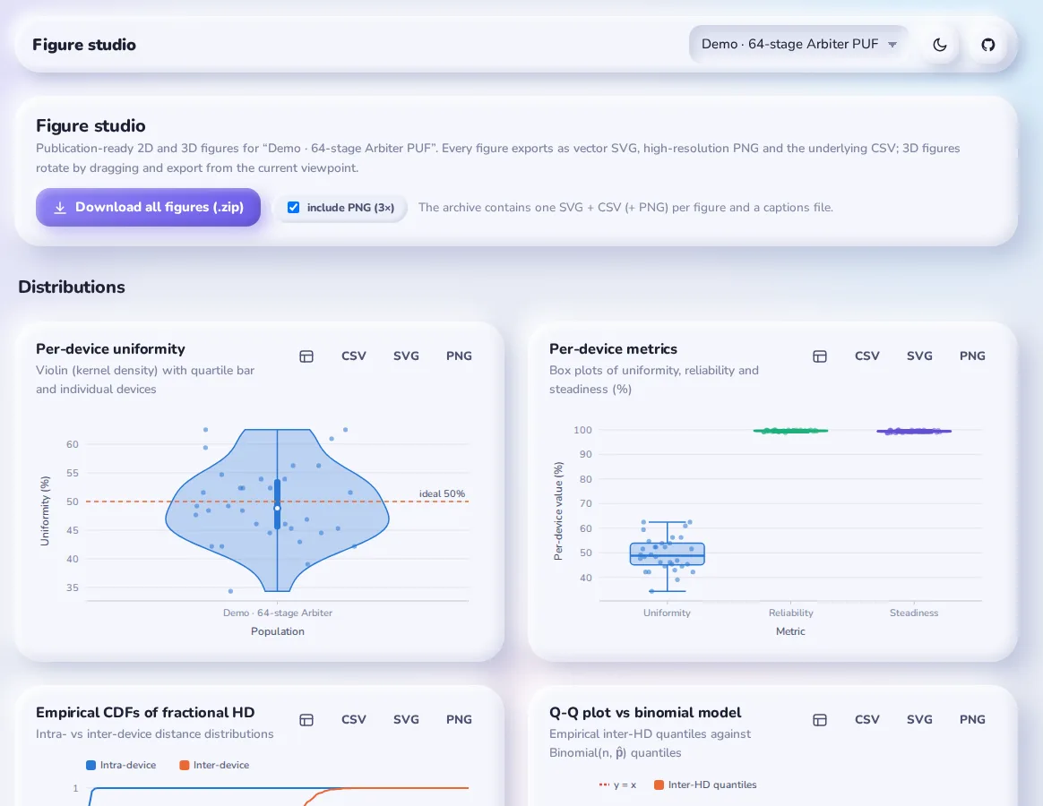
The figure studio draws publication-ready figures from the active data set. Download all figures (.zip) bundles them into one archive: an SVG and a CSV for every figure, a PNG at 3× resolution if you tick include PNG, and a captions file.
| Group | Figures |
|---|---|
| Distributions | per-device uniformity (violin), box plots of per-device metrics, ECDFs of intra/inter distances, Q-Q plot against the binomial model, per-device BER by condition |
| Identification & reliability | ROC curve, identification error vs response length, temporal majority voting (TMV), bit-stability profile |
| Bit-level structure | polar bit-aliasing, entropy accumulation, bias vs instability per bit, uniformity vs reliability per device |
| 3D | stability landscape (flip rate per device × bit), device quality space, inter-device distance bars, identification design space, key-failure surface |
The temporal majority voting figure answers a practical question: if the device reads each bit m times and takes the majority, how much does the error drop? For a cell that flips with probability p, the leftover error is P[Binomial(m, p) > m/2], averaged over all cells. For the demo it falls from 0.38% with one read to 0.10% with fifteen.
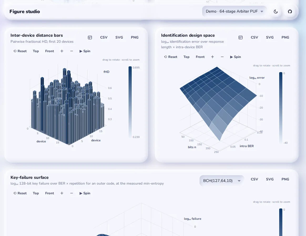
The 3D figures are drawn as SVG with no library behind them. Drag to rotate, scroll to zoom, or use Reset, Top, Front and Spin. The export is whatever view you are looking at. Method notes: figure studio. In Python: quality.tmv_ber() and stats.identification_vs_length().
6. Simulation studio
How does reliability change as noise grows? How many devices do you need before uniqueness settles? The simulation studio runs Monte-Carlo sweeps to find out.
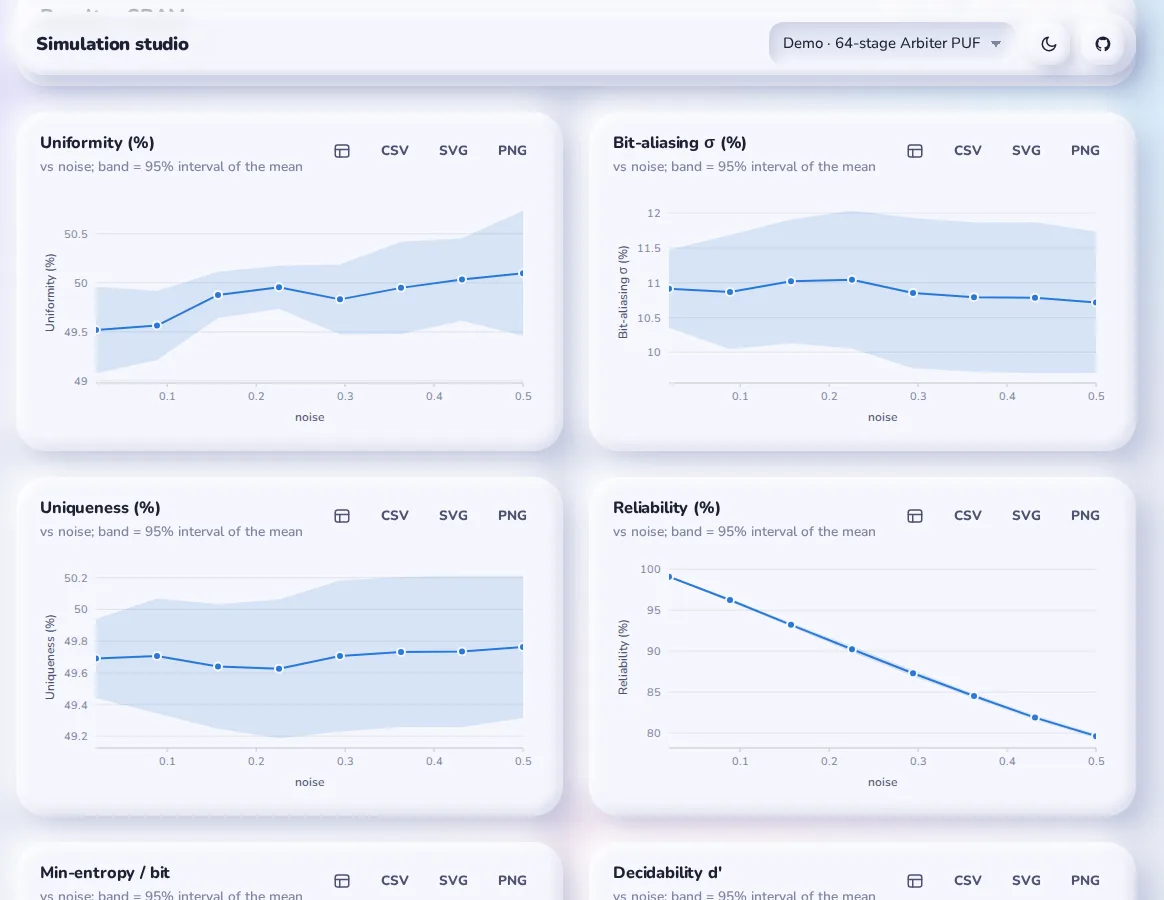
To run a sweep:
- Pick a model and set the population: Devices, Response bits and Repeats.
- Set Seeds per point and First seed.
- Choose Sweep parameter 1, which becomes the x-axis. Any model parameter can be swept, and so can the population size, the response length or the number of repeats.
- Enter its values in one of three forms:
- a list, such as
0.01,0.05,0.1; - a range,
start:stop:steps, such as0.02:0.5:8; - a log range,
log:start:stop:steps.
- a list, such as
- Optionally, choose a second parameter. That turns every metric into a 3D response surface.
Press Run sweep. The cost line shows how many simulations it will take.
Each grid point is simulated with every seed, and the result is the mean with a 95% band, mean ± 1.96·sd/√R for R seeds. The sweep uses common random numbers: replicate r gets seed s₀ + r at every grid point. Neighbouring points then differ only in the parameter, not in the luck of the draw, so the curves come out smooth with few seeds.
In the screenshot, SRAM reliability falls almost linearly from 100% to 80% as noise rises to 0.5, while uniqueness and uniformity do not move. Noise costs you reliability, not uniqueness.
CSV and Python script buttons export the sweep, and pa.sweep() runs the identical computation in Python. Method notes: simulation studio.
7. Attack lab
A PUF that a machine-learning model can predict is not a PUF. The attack lab runs the classic modelling attack: ridge-regularised logistic regression, fitted with Newton’s method, on the challenge-parity features φ(c) of the additive delay model.
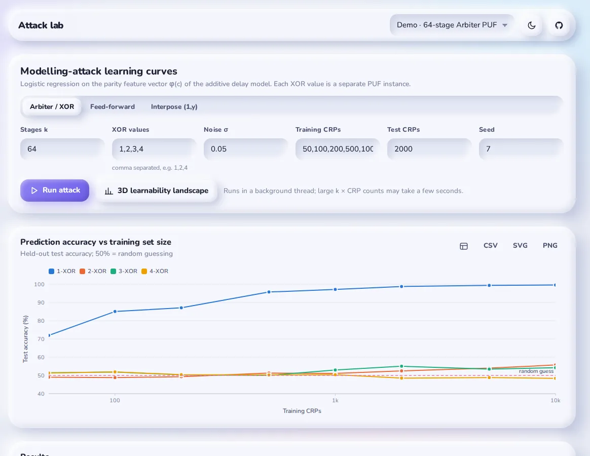
To run it:
- Pick Arbiter / XOR, Feed-forward or Interpose (1,y).
- Set the number of stages.
- List the variants to compare: XOR widths, loop counts or y values, such as
1,2,3,4. - Set the noise, the training set sizes and the test set size.
- Press Run attack.
Each variant is a fresh simulated PUF, and the chart shows its accuracy on held-out challenges as the training set grows. With the defaults:
| PUF | 100 CRPs | 1,000 CRPs | 10,000 CRPs |
|---|---|---|---|
| 64-stage Arbiter (1-XOR) | 85.0% | 97.2% | 99.6% |
| 2-XOR | 48.8% | 51.1% | 55.8% |
| 3-XOR | 51.8% | 53.0% | 54.3% |
| 4-XOR | 51.9% | 50.4% | 48.4% |
A plain Arbiter PUF is broken with a few thousand challenge-response pairs (CRPs). XOR versions stay near 50%, which is guessing, because XORing chains makes the problem non-linear in φ and this learner can only draw a straight boundary.
This shows resistance to this attack only. Neural networks, CMA-ES and reliability-based attacks do break XOR Arbiter PUFs, and the app’s method notes say so.
Two more tools sit below the chart:
- 3D learnability landscape plots accuracy over the number of stages and the training set size.
- Attack your own CRPs takes pasted
challenge,responselines, or the active simulated Arbiter data set, and runs the same attack on your own data.
Method notes: modelling attacks. In Python: attacks.simulated_attack(), attacks.modeling_attack() and attacks.logistic_regression().
8. Key generation
To turn a noisy PUF response into a stable cryptographic key, you need a fuzzy extractor. It combines an error-correcting code with helper data that is stored in public and lets the device repair its noisy read. The planner sizes one.
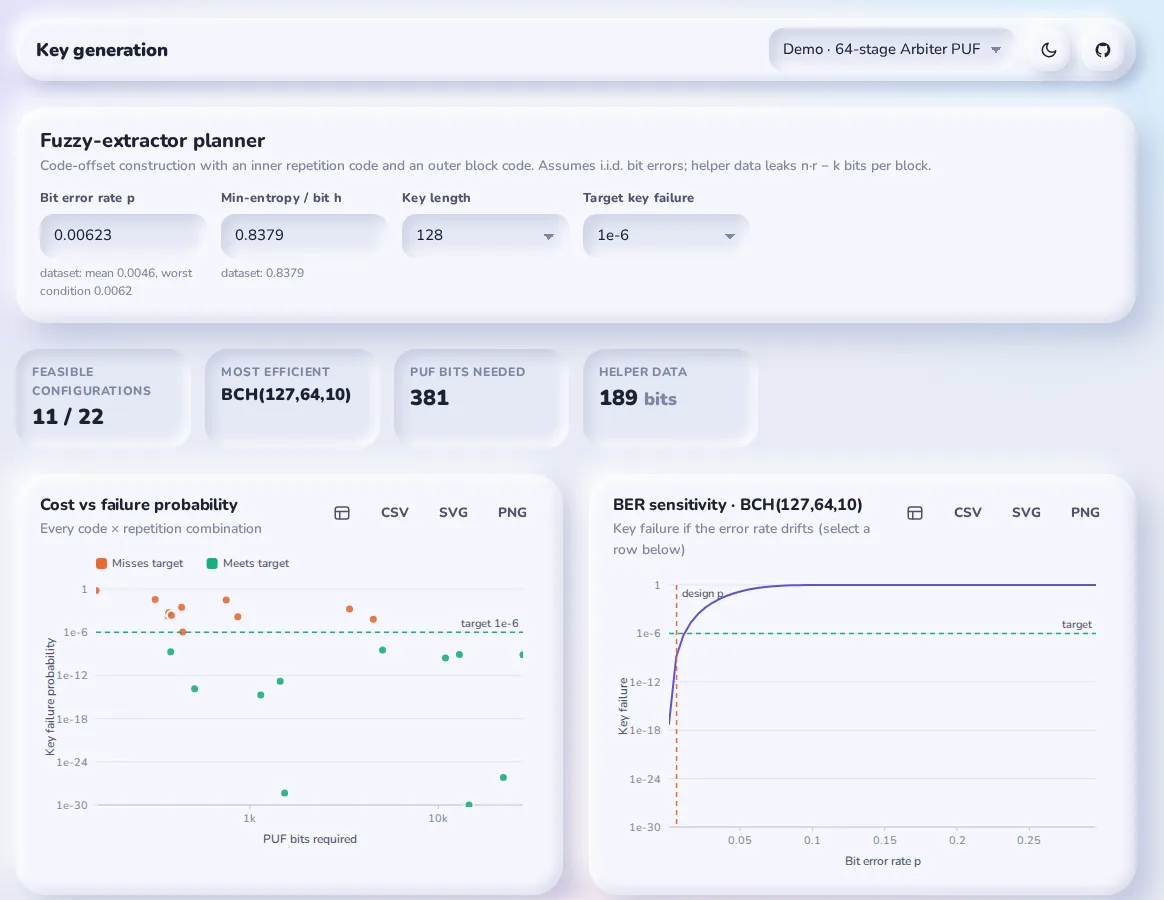
To use it:
- Enter four numbers: the bit error rate p, the min-entropy per bit h, the key length (64 to 256 bits) and the target key failure (10−3 to 10−12).
- When a data set is loaded, the form suggests its own values. Use the worst operating condition’s BER for a conservative design.
The planner tries every combination of an inner repetition code (r = 1 to 15) and an outer block code (Hamming, Golay, Reed–Muller or BCH). It then lists the feasible ones, cheapest first. It uses the code-offset model:
Each block of nr PUF bits leaks nr − k bits through the helper data, which leaves nrh − (nr − k) bits of entropy. The number of blocks B is chosen so that the leftover entropy covers the key.
For the demo, with a worst-case BER of 0.62%, h = 0.838 and a 128-bit key at 10−6, the winner is BCH(127,64,10) with no repetition. It needs 3 blocks, 381 PUF bits and 189 helper bits, and its failure rate is 1.9 × 10⁻⁹.
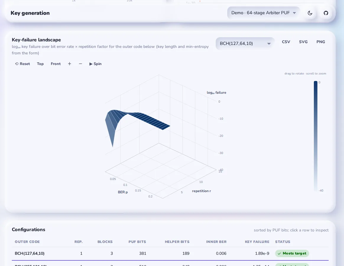
The cost vs failure scatter plots every configuration, and the BER sensitivity curve shows how fast the selected design fails if the error rate drifts. The 3D landscape shows the same thing over BER and repetition at once. Click any row of the table to inspect it.
The model assumes independent bit errors and ignores decoder-specific and side-channel leakage. Method notes: key generation. In Python: ecc.plan_key_generation(), ecc.repetition_error() and ecc.block_failure().
9. Compare
Load or simulate two or more data sets, and Compare puts them side by side. Tick the data sets to include.
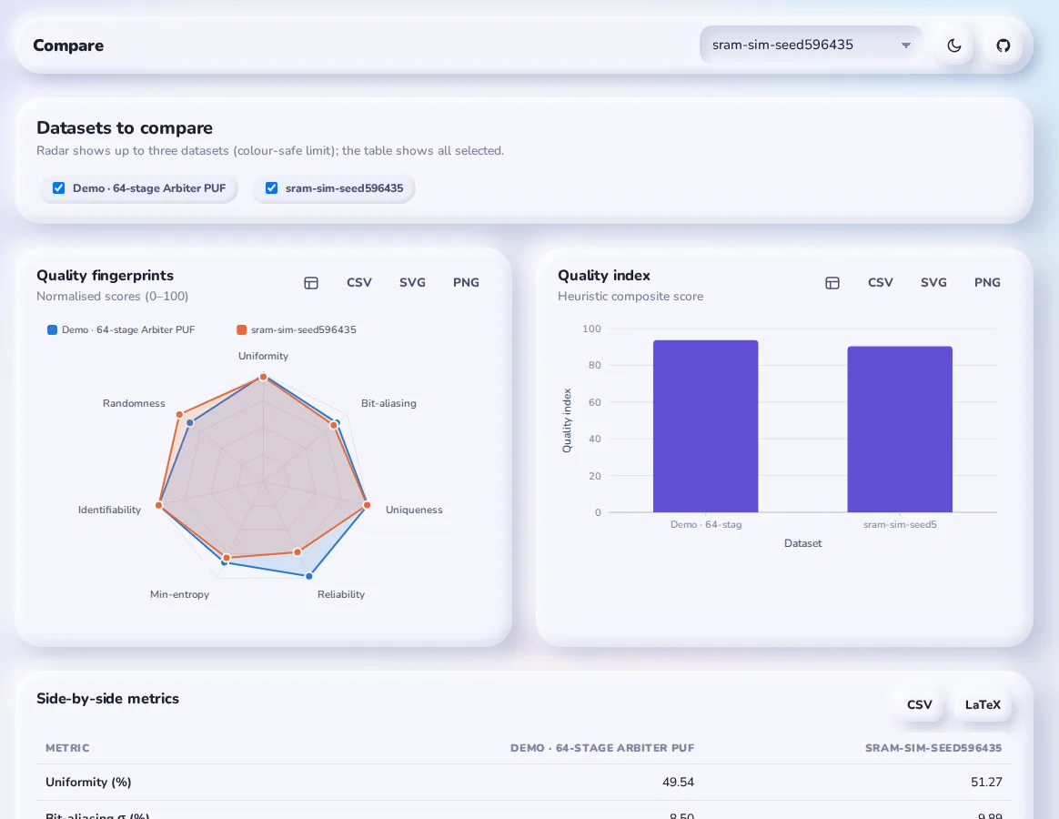
The radar overlays up to three data sets; more would no longer be readable in colour. The quality index bar chart and the side-by-side table show all selected data sets, and the table exports as CSV or LaTeX. The usual use is comparing designs (Arbiter against SRAM against RO) or batches (two wafers, two temperatures).
The quality index is the mean of seven normalised scores, which the radar also shows:
- uniformity;
- bit-aliasing;
- uniqueness;
- reliability;
- min-entropy;
- identifiability, from d′;
- the share of NIST tests passed.
It is a navigation aid, not a standard. The app says so, and so do I: report the individual metrics in papers. Method notes: quality index.
10. Report & export
Everything you need to publish and reproduce the evaluation, in one place:
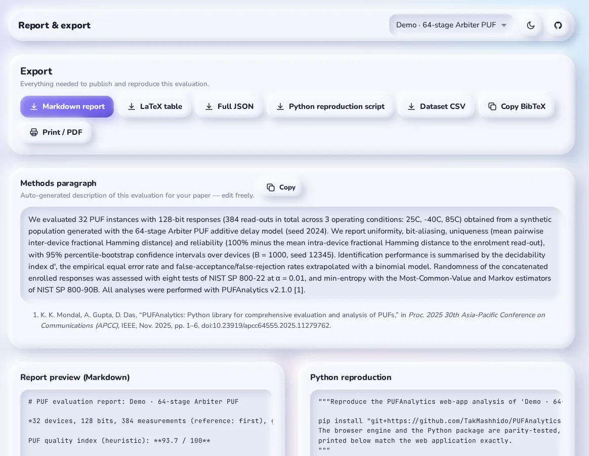
- Markdown report: every metric, readable.
- LaTeX table: a
booktabstable of the headline metrics, ready for\input{}. - Full JSON: every number, per device and per bit. The structure is identical to the one Python’s
pa.analyze()returns. - Python reproduction script: a short
.pyfile that loads the exported CSV with your exact settings and recomputes everything. A reviewer can check your numbers without opening a browser. - Dataset CSV: the data in the long format above.
- Copy BibTeX and Print / PDF.
- Methods paragraph: written from your actual data set and settings, with references, ready to edit and paste into the paper.
11. Methods & docs
The last view is the reference manual: every definition, estimator and assumption behind the numbers, with formulas typeset in KaTeX.
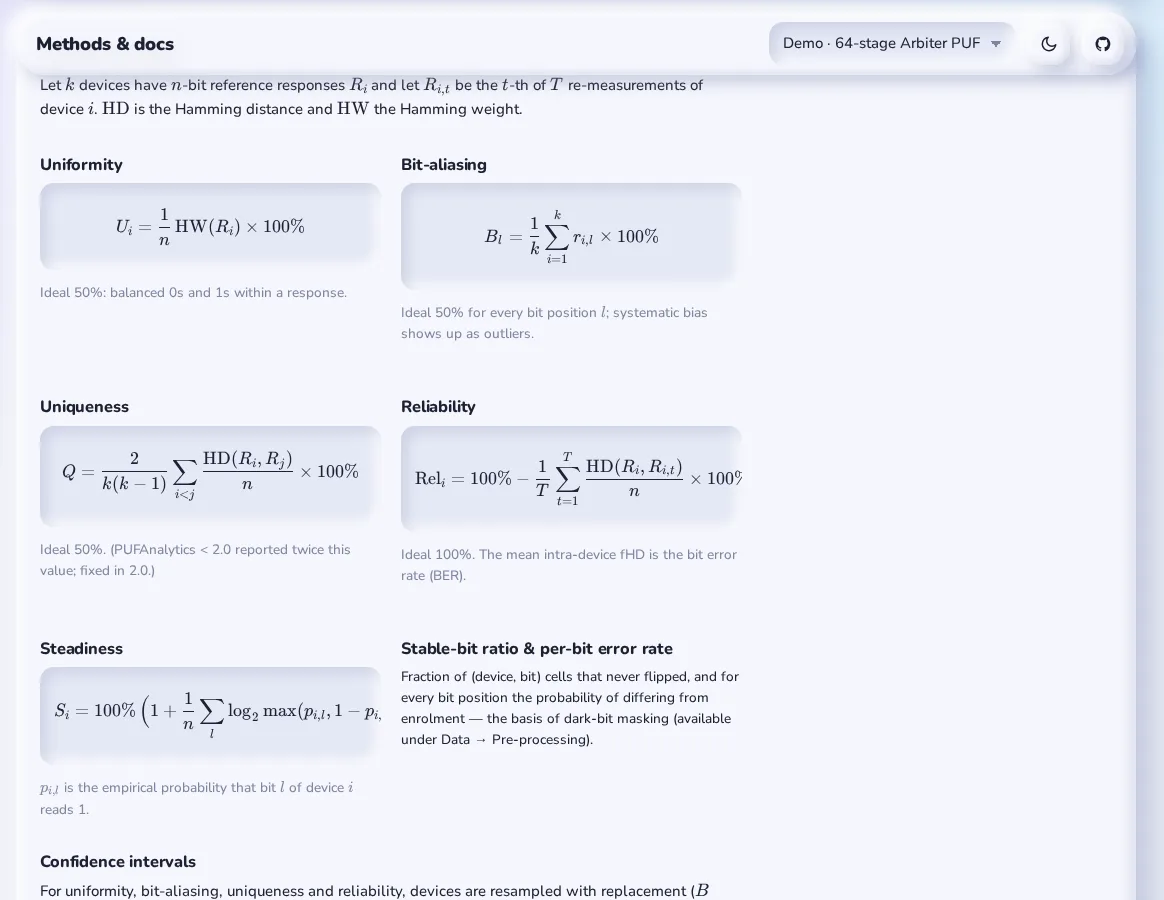
Each section has its own link, so you can cite exactly the part you mean:
| Section | Link |
|---|---|
| Getting started | #/docs/start |
| Data formats | #/docs/formats |
| Quality metrics and confidence intervals | #/docs/metrics |
| Identification statistics | #/docs/identification |
| Randomness tests and entropy | #/docs/randomness |
| Simulators | #/docs/simulators |
| Figure studio, TMV and sweeps | #/docs/figures |
| Modelling attacks | #/docs/attack |
| Key generation | #/docs/ecc |
| Quality index | #/docs/index |
| Python package and CLI | #/docs/python |
| References and citation | #/docs/refs |
Reproducibility: same seed, same bits
A simulated result is only reproducible if someone else can simulate the same population. Saying “we simulated 32 Arbiter PUFs with noise 0.06” is not enough, because a different random generator gives different chips, and different numbers. PUFAnalytics makes the seed the whole story:
Scroll sideways to see the whole diagram.
pa.simulate(..., seed=2024). Shown here for the demo population: 32 devices, 12 read-outs, 128 challenges on a 64-stage Arbiter PUF.Two details make this hold across languages. xoshiro128** uses only 32-bit integer operations, which JavaScript does exactly with Math.imul and >>> 0. And normal variates use only the cosine branch of Box–Muller, so every normal uses exactly two uniforms and the stream never goes out of step.
The proof is in the numbers. These are the demo population’s results in the browser (from the screenshots above), next to the same population rebuilt in Python with pa.simulate("arbiter", n_devices=32, n_bits=128, n_repeats=4, seed=2024, ...):
| Result | Web app | Python |
|---|---|---|
| Uniformity | 49.54% (CI 47.29–51.78) | 49.5361% (CI 47.2894–51.7822) |
| Uniqueness | 50.13% (CI 49.23–50.85) | 50.1276% (CI 49.2266–50.8494) |
| Reliability | 99.54% (CI 99.44–99.64) | 99.5361% (CI 99.4363–99.6404) |
| Decidability d′ | 11.61 | 11.6054 |
| Binomial FAR at t* = 16 | 2.49 × 10⁻¹⁹ | 2.4935 × 10⁻¹⁹ |
| NIST Serial p-values | 0.0623 / 0.0037 | 0.06228 / 0.00372 |
| Best key design | BCH(127,64,10), 381 bits, 1.89 × 10⁻⁹ | BCH(127,64,10), 381 bits, 1.89 × 10⁻⁹ |
The bootstrap intervals match too. They come from the same seeded generator, so the 1,000 resamples are the same 1,000 resamples.
Using the Python package
pip install "git+https://github.com/TakMashhido/PUFAnalytics.git"It needs Python 3.8 or newer and NumPy, nothing else. SciPy is only used by the test suite, to cross-check the special functions.
Quick start
import pufanalytics as pa

# Real data: device,measurement,condition,response (binary or hex)
ds = pa.PUFDataset.from_file("measurements.csv")

# ...or the demo population from the web app, bit for bit
ds = pa.simulate("arbiter", n_devices=32, n_bits=128, n_repeats=4, seed=2024,
                 conditions=[("25C", 1.0), ("-40C", 1.8), ("85C", 2.6)],
                 stages=64, xor=1, noise=0.06)

result = pa.analyze(ds, reference="first", bootstrap=1000, seed=12345)
print(pa.to_markdown(result))           # readable report
pa.to_latex(result, "puf_table.tex")    # booktabs table for the paper
pa.to_json(result, "puf_full.json")     # every number, per device and per bit
pa.analyze() runs everything the web app’s views show and returns a plain dictionary. Its main keys are uniformity, uniqueness, reliability, ber, conditions, identification, entropy, nist, correlation and confidence_intervals.
Building blocks
Each analysis is also available on its own:
from pufanalytics import quality, stats, nist, estimators, attacks, ecc
import pufanalytics as pa

quality.uniqueness(ds)                  # % (ideal 50)
quality.reliability(ds)                 # % per device
quality.bit_flip_rate(ds)               # per-bit error rate, for dark-bit masking
quality.condition_ber(ds)               # {'25C': {'ber': 0.0024, ...}, '85C': {'ber': 0.0062, ...}}
quality.tmv_ber(ds)                     # BER after temporal majority voting
nist.run_all(ds.reference().ravel())    # the eight SP 800-22 tests
estimators.markov_min_entropy(ds.reference().ravel())
stats.identification_vs_length(0.05, 0.5, [64, 128, 256])
pa.sweep("sram", "noise", [0.05, 0.1, 0.2], param2="n_bits", values2=[64, 128], seeds=5)
attacks.simulated_attack(stages=64, xor=2, train_sizes=(100, 1000, 10000))
ecc.plan_key_generation(ber=0.0062, min_entropy=0.838, key_bits=128, target_failure=1e-6)
Command line
Installing the package also installs a pufanalytics command:
| Command | What it does |
|---|---|
pufanalytics simulate MODEL -o out.csv | Simulate a population. Options: --devices, --bits, --repeats, --seed, --conditions 25C:1,85C:2.5 and repeatable --param key=value (such as --param xor=2). Writes .csv or .json. |
pufanalytics analyze FILE | Run the full evaluation. Options: --markdown, --latex and --json to save reports, --reference first|majority, --bootstrap, --seed, --no-nist and --format auto|bin|hex. |
pufanalytics nist FILE | Print the SP 800-22 results for the enrolled responses (--alpha, --reference). |
pufanalytics attack | Logistic-regression learning curve on a simulated Arbiter PUF (--stages, --xor, --noise, --train-sizes, --test-size, --seed). |
pufanalytics ecc --ber P | Fuzzy-extractor plans (--min-entropy, --key-bits, --target, --top). |
pufanalytics simulate sram -o sram.csv --devices 50 --bits 256 --conditions 25C:1,85C:2.5 --param bias=0.1
pufanalytics analyze sram.csv --markdown report.md --latex table.tex --json full.json
pufanalytics ecc --ber 0.0062 --min-entropy 0.838 --key-bits 128 --target 1e-6
The original v1 string-based functions (hamming_distance, uniqueness and the rest) still work unchanged, so old scripts keep running. One exception is uniqueness, which now follows the standard definition, as described above.
Full Python API reference
Every public function, class and method in the package is listed below, generated from the source code itself. Each name links to its definition on GitHub, pinned to the v2.1.0 commit, and each module links to the method notes that explain it. Open a module to see its functions.
pufanalytics.reportOne-call analysis and reports5
| Name | What it does |
|---|---|
analyze(data, reference='first', bootstrap=1000, seed=12345, alpha=0.05, …) | Run the complete PUFAnalytics evaluation. |
to_json(result, path=None, indent=2) | Serialise an analyze result (NaN/inf -> null). |
headline_rows(r) | Rows (metric, value, ideal, CI) shared by Markdown and LaTeX output. |
to_markdown(result, path=None) | Render an analyze result as a Markdown report. |
to_latex(result, path=None, caption=None, label='tab:puf-metrics') | Render the headline metrics as a LaTeX table (booktabs). |
pufanalytics.datasetLoading and shaping data17
| Name | What it does |
|---|---|
parse_response(token, fmt='auto') | Convert a textual response into a uint8 bit vector. |
parse_text(text, fmt='auto') | Parse a textual data set. |
PUFDataset(responses, device_ids=None, conditions=None, challenges=None, …) | Container for PUF response measurements. |
PUFDataset.n_devices | Number of devices (property). |
PUFDataset.n_bits | Response length in bits (property). |
PUFDataset.n_measurements | Read-outs per device, as a list (property). |
PUFDataset.has_repeats | True when any device was measured more than once (property). |
PUFDataset.condition_labels | Operating-condition labels in first-seen order (property). |
PUFDataset.reference(method='first') | Enrolled reference response of every device, shape (devices, bits). |
PUFDataset.to_array() | Return a (devices, measurements, bits) array (rectangular data only). |
PUFDataset.subset(devices=None, bits=None) | Return a new data set restricted to the given device / bit indices. |
PUFDataset.from_bitstrings(responses, **kw) | One response string per device. |
PUFDataset.from_text(text, fmt='auto', name=None) | Build a data set from CSV/TXT text (see parse_text). |
PUFDataset.from_file(path, fmt='auto') | Load a .csv/.txt (see parse_text), .npy or .json file. |
PUFDataset.to_csv(path=None, fmt='bin') | Write the long device,measurement,condition,response format. |
PUFDataset.to_dict() | Plain dict for JSON export; the web app imports it. |
PUFDataset.from_dict(obj) | Rebuild a data set from to_dict() output. |
pufanalytics.qualityQuality metrics18
| Name | What it does |
|---|---|
as_dataset(data) | Coerce supported inputs into a PUFDataset. |
uniformity(data, reference='first') | Uniformity (fraction of 1s, %) of each device's reference response. Ideal 50 %. |
bit_aliasing(data, reference='first') | Bit-aliasing (%) per bit position across devices. Ideal 50 %. |
inter_hd_matrix(data, reference='first') | Symmetric devices x devices matrix of inter-device Hamming distances. |
inter_hd(data, reference='first') | All pairwise inter-device Hamming distances (integer), upper triangle. |
uniqueness(data, reference='first') | Uniqueness: mean pairwise inter-device fHD in %. Ideal 50 %. |
intra_hd(data, reference='first') | Intra-device Hamming distances between the reference and every re-measurement. |
reliability(data, reference='first') | Reliability (%) per device: 100 - mean intra fHD * 100. Ideal 100 %. |
steadiness(data) | Steadiness (%) per device (Maiti et al.): 100 (1 + mean_l log2 max(p_l, 1-p_l)). |
bit_flip_rate(data, reference='first') | Per-bit error rate: probability that bit l differs from the reference. |
stable_bit_ratio(data) | Fraction of (device, bit) cells that never changed over all measurements. |
condition_ber(data) | Mean bit error rate w.r.t. the enrolment read-out, per operating condition. |
hamming_weights(data, reference='first') | Hamming weight of every device's reference response. |
bit_correlation_matrix(data, reference='first', max_bits=256) | Pearson (phi) correlation between bit positions across devices. |
autocorrelation(data, reference='first', max_lag=32) | Mean normalised autocorrelation of the reference responses (±1 mapping). |
bit_entropy(data, reference='first') | Shannon entropy (bits) of every bit position across the device population. |
bit_min_entropy(data, reference='first') | Min-entropy (bits) of every bit position across the device population. |
tmv_ber(data, votes=(1, 3, 5, 7, 9, 11, 13, 15)) | Bit error rate after temporal majority voting (TMV) over m read-outs. |
pufanalytics.statsStatistics and identification16
| Name | What it does |
|---|---|
igam(a, x) | Regularised lower incomplete gamma function P(a, x). |
igamc(a, x) | Regularised upper incomplete gamma function Q(a, x) = 1 - P(a, x). |
normal_cdf(x) | Standard normal cumulative distribution function. |
binom_logpmf(k, n, p) | Natural log of the binomial probability mass function. |
binom_pmf_vector(n, p) | Return the binomial pmf for k = 0..n as a NumPy array. |
binom_cdf(k, n, p) | P(X <= k) for X ~ Binomial(n, p), accurate deep into the tails. |
binom_sf(k, n, p) | P(X > k) for X ~ Binomial(n, p), accurate deep into the tails. |
decidability(intra, inter) | Decidability index d' (Daugman) between intra- and inter-distance sets. |
histogram_counts(hd_values, n_bits) | Histogram of integer Hamming distances on the support 0..n_bits. |
far_frr_curve(intra_hd, inter_hd, n_bits) | Empirical FAR / FRR as a function of the HD acceptance threshold. |
equal_error_rate(far, frr) | Equal error rate and the threshold index where it is attained. |
binomial_fit(hd_values, n_bits) | Fit a binomial model Binomial(n_bits, p) to Hamming distances. |
binomial_far_frr(n_bits, p_intra, p_inter) | FAR / FRR under the independent-bit binomial model. |
percentile_ci(samples, alpha=0.05) | Two-sided percentile confidence interval of bootstrap replicates. |
bootstrap_indices(n, n_resamples, seed=0) | Generate bootstrap index sets with the portable RNG (reproducible). |
identification_vs_length(p_intra, p_inter, lengths) | Binomial-model identification error min_t max(FAR, FRR) for each response length. |
pufanalytics.nistNIST SP 800-22 randomness tests9
| Name | What it does |
|---|---|
monobit(seq, alpha=0.01, strict=True) | 2.1 Frequency (monobit) test. Requires n >= 100. |
block_frequency(seq, alpha=0.01, block_size=None, strict=True) | 2.2 Frequency test within a block. Requires n >= 100. |
runs(seq, alpha=0.01, strict=True) | 2.3 Runs test. Requires n >= 100. |
longest_run(seq, alpha=0.01, strict=True) | 2.4 Test for the longest run of ones in a block. Requires n >= 128. |
cumulative_sums(seq, alpha=0.01, strict=True) | 2.13 Cumulative sums (forward and backward). Requires n >= 100. |
approximate_entropy(seq, alpha=0.01, m=None, strict=True) | 2.12 Approximate entropy test. Requires m < floor(log2 n) - 5. |
serial(seq, alpha=0.01, m=None, strict=True) | 2.11 Serial test (two p-values). Requires m < floor(log2 n) - 2. |
spectral(seq, alpha=0.01, strict=True) | 2.6 Discrete Fourier transform (spectral) test. Requires n >= 1000. |
run_all(seq, alpha=0.01, strict=True) | Run every implemented SP 800-22 test and return a list of results. |
pufanalytics.estimatorsEntropy estimators5
| Name | What it does |
|---|---|
shannon_entropy_rate(seq) | Shannon entropy (bits per bit) of the empirical 0/1 distribution. |
mcv_min_entropy(seq) | SP 800-90B Most Common Value min-entropy estimate (bits per bit). |
markov_min_entropy(seq, length=128) | SP 800-90B Markov min-entropy estimate for binary data (bits per bit). |
lz_complexity(seq) | Normalised Lempel-Ziv (1976) complexity c(n) log2(n) / n. |
population_entropy(data, reference='first') | Summary of per-position entropy across a device population. |
pufanalytics.simulatorsPUF simulators3
| Name | What it does |
|---|---|
arbiter_features(challenges) | Parity feature transform of the additive delay model. |
ff_loops(stages, loops) | (source, destination) stage pairs of evenly spaced, non-overlapping feed-forward loops. |
simulate(model='arbiter', n_devices=20, n_bits=128, n_repeats=5, seed=1, …) | Simulate a PUF population. |
pufanalytics.sweepMonte-Carlo sweeps2
| Name | What it does |
|---|---|
quick_metrics(ds) | Fast headline metrics (no bootstrap, no NIST) used by sweeps. |
sweep(model='arbiter', param='noise', values=(0.01, 0.05, 0.1), …) | Sweep one (or two) simulator parameters. |
pufanalytics.attacksModelling attacks3
| Name | What it does |
|---|---|
logistic_regression(X, y, l2=0.01, max_iter=30, tol=1e-06) | Fit ridge-regularised logistic regression with Newton's method. |
modeling_attack(challenges, responses, train_sizes=(50, 100, 200, 500, 1000, …) | Learning curve of a logistic-regression attack on supplied CRPs. |
simulated_attack(stages=64, xor=1, noise=0.05, train_sizes=(50, 100, 200, 500, …) | Learning curve of the attack against a simulated (k-XOR) Arbiter PUF. |
pufanalytics.eccKey generation planning3
| Name | What it does |
|---|---|
repetition_error(p, r) | Residual bit error after majority decoding of an (r,1) repetition code. |
block_failure(p, n, t) | Probability that a block of n bits has more than t errors. |
plan_key_generation(ber, min_entropy=1.0, key_bits=128, target_failure=1e-06, …) | Enumerate ECC configurations and report the feasible ones. |
pufanalytics.rngPortable random number generator9
| Name | What it does |
|---|---|
PortableRNG(seed=0) | xoshiro128** generator with a SplitMix32 seeder. |
PortableRNG.next_u32() | Return the next unsigned 32-bit integer. |
PortableRNG.random() | Uniform double in [0, 1). |
PortableRNG.bit() | A single fair random bit (the most significant bit of the output). |
PortableRNG.normal() | Standard normal variate (Box-Muller, cosine branch). |
PortableRNG.randint(n) | Uniform integer in [0, n). |
PortableRNG.bits(count) | Return a list of count fair bits. |
PortableRNG.normals(count) | Return a list of count standard normal variates. |
PortableRNG.randoms(count) | Return a list of count uniform doubles in [0, 1). |
pufanalytics.cliCommand line1
| Name | What it does |
|---|---|
main(argv=None) | Entry point of the pufanalytics command (analyze, simulate, nist, attack, ecc). |
pufanalytics.metricsOriginal string API (v1, kept for compatibility)13
| Name | What it does |
|---|---|
hamming_distance(seq1, seq2) | Compute the Hamming distance between two sequences of equal length. |
bit_error_rate(expected, actual) | Compute the bit error rate between two sequences of equal length. |
intra_puf_variation(responses) | Compute the intra-PUF variation. |
inter_puf_variation(puf_responses) | Compute the inter-PUF variation. |
uniqueness(puf_responses) | Compute the uniqueness metric for a list of PUF responses. |
reliability(responses) | Compute the reliability of a list of PUF responses. |
avalanche_effect(responses) | Compute the avalanche effect for a list of PUF responses. |
uniformity(response) | Compute the uniformity of a single PUF response. |
bit_aliasing(responses) | Compute the bit aliasing for a list of PUF responses. |
correlation_coefficient(response) | Compute the correlation coefficient between PUF responses. |
entropy(puf_responses) | Compute the entropy of a list of PUF responses. |
mutual_information(puf_responses) | Compute the mutual information between PUF responses. |
min_entropy(puf_responses) | Compute the min-entropy of a list of PUF responses. |
How it is tested
- NIST worked examples. Each SP 800-22 test reproduces the example sequences and p-values printed in the standard, to six decimal places.
- SciPy cross-checks. The incomplete gamma functions, normal CDF and binomial tails are compared against SciPy to about 10−12 relative error, including far tails.
- Cross-language parity. The over 2,400 values in
golden.json, from Python, must be reproduced by the browser engine: simulated populations bit for bit, and statistics to floating-point tolerance. - Continuous integration runs the pytest suite and the parity test on every push. A separate workflow deploys the web app to GitHub Pages.
pytest -q                          # Python test suite
python tests/make_golden.py        # regenerate reference values from Python
node web/tests/parity.test.mjs     # the browser engine must match them
What it does not do
- It assumes independent bit errors in the binomial identification model and in the key planner. Real PUFs often have correlated errors, for example cells that fail together when hot. Check the χ² fit p-value; when it is tiny, trust the empirical curves more than the extrapolated ones.
- A resisted attack is not a security proof. The attack lab runs one classic learner. It is useful for showing why XOR helps, and useless for claiming that something is secure.
- The quality index is a heuristic. It helps you compare designs at a glance. Do not put it in a paper as a metric.
- The simulators are models, not silicon. They are good for intuition, for checking the pipeline, and for “what if” sweeps. They do not replace measuring real chips.
Citing PUFAnalytics
If PUFAnalytics helps your research, please cite the paper:
K. K. Mondal, A. Gupta and D. Das, “PUFAnalytics: Python Library for Comprehensive Evaluation and Analysis of PUFs,” 2025 30th Asia-Pacific Conference on Communications (APCC), IEEE, 2025, pp. 1–6, doi: 10.23919/apcc64555.2025.11279762.
The Copy BibTeX button in the app, and CITATION.cff in the repository, have the BibTeX entry.
Links
- Web app: koustav.isroot.in/PUFAnalytics, and its Methods & docs
- Source, issues and changelog: github.com/TakMashhido/PUFAnalytics
- The paper: doi:10.23919/apcc64555.2025.11279762
- Background: How a PUF works, from silicon variation to a login protocol
- The standards: NIST SP 800-22 rev. 1a (randomness tests) and SP 800-90B (entropy estimation)